import numpy as np  #Numeric Python
import pandas as pd #Data structures & anaylysis
import matplotlib   #Plotting and visualization
import matplotlib.pyplot as plt
import datetime as dt#Datatype to hold timestamps
#Magic function to enable inline plots in ipython
%matplotlib inline
 .
.![1]: https://www.ncdc.noaa.gov/crn/qcdatasets.html
dateparse = lambda x: pd.datetime.strptime(x, '%Y%m%d %H%M')
inputFile='CRNS0101-05-2016-OK_Stillwater_2_W.csv'
df = pd.read_csv(inputFile)

df['LST_TIME']=[str(x).zfill(4) for x in df['LST_TIME']]
df['timestamp']=[str(x)+' '+str(y) for x,y in zip(df['LST_DATE'],df['LST_TIME'])]
df['timestamp']=[str(x).strip('\n') for x in df['timestamp']]
df['timestamp']=df['timestamp'].apply(lambda x: dt.datetime.strptime(x,'%Y%m%d %H%M'))
df.to_csv('temperature_data_stillwater_OK_2_W.csv')


#print (df['timestamp'][0])
temperatureDF=pd.DataFrame()
temperatureDF['timestamp']=df['timestamp']
temperatureDF['tempC']=df['AIR_TEMPERATURE']
temperatureDF.to_csv('temperature_data.csv',index=False)
temperatureDateConverter = lambda d : dt.datetime.strptime(d.decode("utf-8"),'%Y-%m-%d %H:%M:%S')
temperature = np.genfromtxt('temperature_data.csv',delimiter=",",dtype=[('timestamp', type(dt.datetime.now)),('tempC', 'f8')],converters={0: temperatureDateConverter}, skip_header=1)
print (temperature)
[(datetime.datetime(2016, 1, 1, 0, 0), -1.8)
 (datetime.datetime(2016, 1, 1, 0, 5), -2.0)
 (datetime.datetime(2016, 1, 1, 0, 10), -1.9) ...,
 (datetime.datetime(2016, 12, 31, 17, 50), 6.3)
 (datetime.datetime(2016, 12, 31, 17, 55), 5.9)
 (datetime.datetime(2016, 12, 31, 18, 0), 5.6)]
print("The variable 'temperature' is a " + str(type(temperature)) + " and it has the following shape: " + str(temperature.shape))
The variable 'temperature' is a <type 'numpy.ndarray'> and it has the following shape: (105337,)
temperature.dtype.fields
<dictproxy {'tempC': (dtype('float64'), 8), 'timestamp': (dtype('O'), 0)}>
#dates = matplotlib.dates.date2num(temperature['timestamp'][0:10])
#tval=[i for i in range(0,10)]
#matplotlib.pyplot.plot_date()
plt.plot(temperature['timestamp'])

#axes = plt.gca()
#plt.gcf().autofmt_xdate()
#axes.set_xlim([xmin,xmax])
#axes.set_ylim([ymin,ymax])
[<matplotlib.lines.Line2D at 0x7f9ec83ede10>]
#ttt=df.to_dict('list')
#print ttt['timestamp']
print("The minimum difference between any two consecutive timestamps is: " + str(np.min(np.diff(temperature['timestamp']))))
print("The maximum difference between any two consecutive timestamps is: " + str(np.max(np.diff(temperature['timestamp'])))      )
The minimum difference between any two consecutive timestamps is: 0:05:00
The maximum difference between any two consecutive timestamps is: 0:05:00
temperature = temperature[0:-1:3]
print("First timestamp is on \t{}. \nLast timestamp is on \t{}.".format(temperature['timestamp'][0], temperature['timestamp'][-1]))
First timestamp is on 	2016-01-01 00:00:00.
Last timestamp is on 	2016-12-31 17:45:00.
dateparse = lambda x: pd.datetime.strptime(x, '%Y%m%d %H%M')
inputFile='data_download.csv'
powerDF = pd.read_csv(inputFile)

powerDF['Meter Read Start']=powerDF['Meter Read Start'].apply(lambda x: dt.datetime.strptime(x.split('.')[0],'%Y-%m-%dT%H:%M:%S'))
powerDF['Meter Read End']=powerDF['Meter Read End'].apply(lambda x: dt.datetime.strptime(x.split('.')[0],'%Y-%m-%dT%H:%M:%S'))
powerDF.to_csv('power_data.csv',index=False)
dateConverter = lambda d : dt.datetime.strptime(d.decode("utf-8"),'%Y-%m-%d %H:%M:%S')
power = np.genfromtxt('power_data.csv',delimiter=",",names=True,dtype=['S255',dt.datetime,dt.datetime,'S255','f8','S255','f8','S255'],converters={1: dateConverter})
print power.dtype.fields
{'Consumption_or_Production_Value': (dtype('float64'), 526), 'Consumption_or_Production': (dtype('S255'), 271), 'Consumption_or_Production_Unit': (dtype('S255'), 534), 'Meter_Read_Start': (dtype('O'), 255), 'Meter_Number': (dtype('S255'), 0), 'Meter_Read_End': (dtype('O'), 263), 'Value': (dtype('float64'), 789), 'Units': (dtype('S255'), 797)}
** Notice ** that the column/header name Time is now going to be Meter_Read_Start moving forward
name, indices, counts = np.unique(power['Meter_Number'], return_index=True,return_counts=True)
for i in range(len(name)):
    print('Meter Number:'+str(name[i])+"\n\t from "+str(power[indices[i]]['Meter_Read_Start'])+" to "+str(power[indices[i]+counts[i]-1]['Meter_Read_Start'])+"\n\t or "+str(power[indices[i]+counts[i]-1]['Meter_Read_Start']-power[indices[i]]['Meter_Read_Start']))
Meter Number:763811062
	 from 2016-03-13 00:00:00 to 2016-12-30 17:45:00
	 or 292 days, 17:45:00
power = np.sort(power,order='Meter_Read_Start')
fig1= plt.figure(figsize=(15,5))
plt.plot(power['Meter_Read_Start'],power['Value'])
plt.title(name[0])
plt.xlabel('Time')
plt.ylabel('Power [Watts]')
<matplotlib.text.Text at 0x7f9ec98932d0>
power = np.sort(power,order='Meter_Read_Start')
print "The minimum difference between any two consecutive timestamps is: " + str(np.min(np.diff(power['Meter_Read_Start'])))
print "The maximum difference between any two consecutive timestamps is: " + str(np.max(np.diff(power['Meter_Read_Start'])))
The minimum difference between any two consecutive timestamps is: 0:00:00
The maximum difference between any two consecutive timestamps is: 2 days, 0:15:00
print "First timestamp is on \t{}. \nLast timestamp is on \t{}.".format(power['Meter_Read_Start'][0], power['Meter_Read_Start'][-1])
First timestamp is on 	2016-03-13 00:00:00.
Last timestamp is on 	2016-12-30 17:45:00.
print "Power data from {0} to {1}.\nTemperature data from {2} to {3}".format(power['Meter_Read_Start'][0], power['Meter_Read_Start'][-1], temperature['timestamp'][0], temperature['timestamp'][-1])
Power data from 2016-03-13 00:00:00 to 2016-12-30 17:45:00.
Temperature data from 2016-01-01 00:00:00 to 2016-12-31 17:45:00
ttt=temperature
temperature = ttt[5246:-24*4]
print "Power data from {0} to {1}.\nTemperature data from {2} to {3}".format(power['Meter_Read_Start'][0], power['Meter_Read_Start'][-1], temperature['timestamp'][0], temperature['timestamp'][-1])
Power data from 2016-03-13 00:00:00 to 2016-12-30 17:45:00.
Temperature data from 2016-02-24 15:30:00 to 2016-12-30 17:45:00
def power_interp(tP, P, tT):
    # This function assumes that the input is an numpy.ndarray of datetime objects

    # Most useful interpolation tools don't work well with datetime objects
    # so I will convert all datetime objects into the number of seconds elapsed
    # since 1/1/1970 at midnight (also called the UNIX Epoch, or POSIX time):

    toposix = lambda d: (d - dt.datetime(1970,1,1,0,0,0)).total_seconds()
    tP = map(toposix, tP)
    tT = map(toposix, tT)

    # Now we interpolate
    from scipy.interpolate import interp1d
    f = interp1d(tP, P,'linear',bounds_error=False)

    return f(tT)
newPowerValues = power_interp(power['Meter_Read_Start'], power['Value'], temperature['timestamp'])
toposix = lambda d: (d - dt.datetime(1970,1,1,0,0,0)).total_seconds()

timestamp_in_seconds = map(toposix,temperature['timestamp'])
timestamps = temperature['timestamp']
temp_values = temperature['tempC']
power_values = newPowerValues
a=(timestamps, power_values, temp_values)
data = np.asarray(a)
data = data.T
print "The size of the data is: " + str((data.shape)) + "and the type is:  " + str(type(data))
print data[0]
The size of the data is: (29770, 3)and the type is:  <type 'numpy.ndarray'>
[datetime.datetime(2016, 2, 24, 15, 30) nan 12.9]
weekday = map(lambda t: t.weekday(), timestamps)
weekends = np.where([item==5 or item==6 for item in weekday])
weekdays = np.where([item ==0 or item==1 or item==2 or item==3 or item==4 for item in weekday])
len(weekday) == len(weekends[0]) + len(weekdays[0]) ## This is assuming you have a tuple of ndarrays
True
hour = map(lambda t: t.hour, timestamps)
unoccupied = np.where([item>=8 and item<=18 for item in hour])
occupied = np.where([item<=8 or item>=18 for item in hour])

#print hour[50:100]
#print occupied[0][0:100]
#print unoccupied[0][0:100]
print power_values
type(power_values)
[  nan   nan   nan ...,  272.  144.  152.]


numpy.ndarray
power_o=power_values[occupied];   # power measurements at occupied times
temp_o=temp_values[occupied];     # temperature measurements at occupied times
power_uo=power_values[unoccupied]; # power measurements at unoccupied times
temp_uo=temp_values[unoccupied];   # temperature measurements at unoccupied times

print str(power_o.shape) + str(power_uo.shape)
(18600,)(13650,)
plt.figure(figsize=(15,15));
f, (ax1, ax2) = plt.subplots(1, 2, sharey=True);
plt.xlabel('temperature');
plt.ylabel('power_measurements');
ax1.plot(temp_o, power_o,'ro');
ax1.set_title('occuppied case');
ax2.plot(temp_uo, power_uo, 'bo');
ax2.set_title('unoccupied case');
plt.xlabel('temperature');
<matplotlib.figure.Figure at 0x7f9ef84fca50>
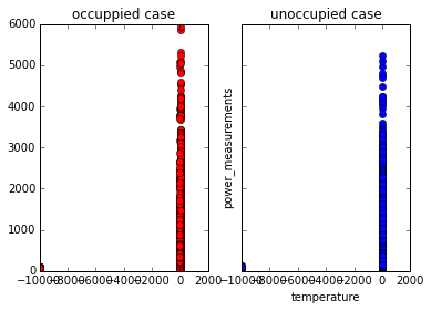
The above figure shows the plot between the power and temperatue in occupied and unoccupied cases.
####
def Tc(temperature, T_bound):
    # The return value will be a matrix with as many rows as the temperature
    # array, and as many columns as len(T_bound) [assuming that 0 is the first boundary]

    Tc_matrix = np.zeros((len(temperature), len(T_bound)))
    for ti in range(0,len(temperature)):
        if temperature[ti]>T_bound[1]:
            Tc_matrix[ti,0]=T_bound[1];

        else:
            Tc_matrix[ti,0]=temperature[ti];
            Tc_matrix[ti,1:]=0;

        for n in range(2,5):
            if temperature[ti]>=T_bound[n]:
                Tc_matrix[ti,n-1]=T_bound[n]-T_bound[n-1]
            else:
                Tc_matrix[ti,n]=temperature[ti]-T_bound[n-1]
                Tc_matrix[ti,n:]=0

        if temperature[ti]>T_bound[5]:# If strictly greater (as in the paper), a temp_value=T_bound[5] will be ignored
            Tc_matrix[ti,4]=T_bound[5]-T_bound[4]
            Tc_matrix[ti,5]=temperature[ti]-T_bound[5]


    return Tc_matrix
Tc_matrix check:
B=(0,10,20,30,40,50)
Tc_mat=Tc(temp_values[0:10],B)
print temp_values[0:10]
print Tc_mat
len(Tc_mat)
[ 12.9  13.2  13.2  13.6  13.7  13.7  13.6  13.5  13.2  12.8]
[[ 10.   0.   0.   0.   0.   0.]
 [ 10.   0.   0.   0.   0.   0.]
 [ 10.   0.   0.   0.   0.   0.]
 [ 10.   0.   0.   0.   0.   0.]
 [ 10.   0.   0.   0.   0.   0.]
 [ 10.   0.   0.   0.   0.   0.]
 [ 10.   0.   0.   0.   0.   0.]
 [ 10.   0.   0.   0.   0.   0.]
 [ 10.   0.   0.   0.   0.   0.]
 [ 10.   0.   0.   0.   0.   0.]]


10
def DesignMatrix(temperature,timestamps,T_bound):
    NumOfWeeks = 28
    model = "unoccupied weekends"
    if model == "full weekdays":
        m = 480
        n = m*NumOfWeeks
    else:
        if model == "full weekends":
            m = 192
            n = m*NumOfWeeks
        else:
            if model == "occupied weekdays":
                m = 5*10*4   # 200
                n = m*NumOfWeeks
            else:
                if model == "unoccupied weekends":
                    m = 112
                    # m = 14 hours per day * 4 intervals per hour * 2 days in a weekend
                    n = m*NumOfWeeks
    p = m-1
    DesignM = np.zeros((n,m+5))
    #DesignM[:,0] = 1
    DesignM[:,0:m]=np.vstack([np.eye(m)]*NumOfWeeks)
    Tc_matrix = Tc(temperature,T_bound)
    DesignM[:,p:]= Tc_matrix

    return DesignM
def beta_hat(DM,power_values):

    #np.linalg.pinv is being used get the pseudo inverse.

    beta_H = (np.linalg.pinv(DM.T.dot(DM)).dot(DM.T).dot(power_values))

    return beta_H
weekday = map(lambda t: t.weekday(), timestamps)
weekdays = np.where([item ==0 or item==1 or item==2 or item==3 or item==4 for item in weekday])
#print weekends[0][1:78]

hour = map(lambda t: t.hour, timestamps)
occupied = np.where([item>=8 and item<=18 for item in hour])

# finding the commen indices between weekends and unoccupied
idx_new = np.intersect1d(weekdays, occupied, assume_unique=False)

type(idx_new)
idx_new.shape
(9778,)
whole_data =(timestamps[idx_new], power_values[idx_new], temp_values[idx_new])
trainData =(whole_data[0][0:5742][:], whole_data[1][0:5742][:], whole_data[2][0:5742][:])
#print len(trainData[0])
testData =(whole_data[0][5742:][:], whole_data[1][5742:][:], whole_data[2][5742:][:])
#print len(testData[0])
timestamps[idx_new].shape
(9778,)
T_lower = min(temp_values[idx_new])
print T_lower
T_upper = max(temp_values[idx_new])
print T_upper
-9999.0
38.7
T_bound = (-10,10,30,50,70,90)
DM = DesignMatrix(trainData[2][0:3136],trainData[0][0:3136],T_bound)
K = DM.T
L=K.dot(DM)
L.shape

#np.linalg.inv

M = np.linalg.pinv(L)
print M.shape

np.linalg.matrix_rank(L)
(117, 117)


113
Beta_coeff = beta_hat(DM,trainData[1][0:3136])
#print Beta_coeff[0:10]
Beta_coeff.shape
(117,)
DM = DesignMatrix(testData[2][0:3136],testData[0][0:3136],T_bound)
Prediction = DM.dot(Beta_coeff)
fig1= plt.figure(figsize=(15,5))
plt.plot(testData[0][0:3136],Prediction[0:3136], 'r')
plt.plot(testData[0][0:3136],testData[1][0:3136], 'b')
plt.title('Predicted and actual value comparison for unoccupied weekdays')
plt.xlabel('Time')
plt.ylabel('Power [Watts]')
<matplotlib.text.Text at 0x7f9ec9e63550>
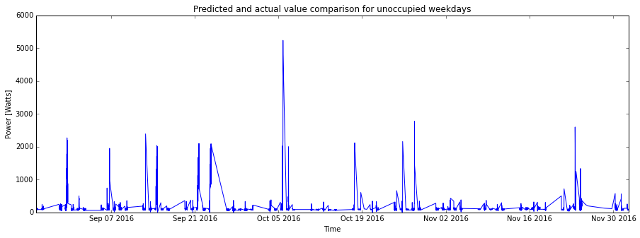
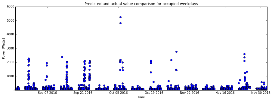
fig1= plt.figure(figsize=(15,5))
plt.plot(testData[0][0:3136],Prediction[0:3136], 'ro')
plt.plot(testData[0][0:3136],testData[1][0:3136], 'bo')
plt.title('Predicted and actual value comparison for occupied weekdays')
plt.xlabel('Time')
plt.ylabel('Power [Watts]')
<matplotlib.text.Text at 0x7f9ec9e32c10>